In the realm of data science and machine learning, understanding statistical results is crucial for making informed decisions. One of the most commonly used packages data scientist encountered daily is statsmodel. Its summary table is a great tool to gain insights to understanding the relationship between explanatory variable and response variable. In this blog post, we’ll dive into how to interpret a Statsmodels summary table and extract meaningful insights from it.
import statsmodels.api as sm
import statsmodels.formula.api as smf
import numpy as np
import pandas
What is a Statsmodels Summary Table?
est  = sm.OLS(y, sm.add_constant(X))
res = est.fit()
print(res.summary())


                            OLS Regression Results
==============================================================================
Dep. Variable:                      y   R-squared:                       0.793
Model:                            OLS   Adj. R-squared:                  0.687
Method:                 Least Squares   F-statistic:                 7.686e+04
Date:                Mon, 18 Dec 2023   Prob (F-statistic):                  0
Time:                        09:29:24   Log-Likelihood:                -375.30
No. Observations:                  85   AIC:                             764.6
Df Residuals:                      78   BIC:                             781.7
Df Model:                           6
Covariance Type:            nonrobust
===============================================================================
                  coef    std err          t      P>|t|      [0.025      0.975]
-------------------------------------------------------------------------------
Intercept      38.6517      9.456      4.087      0.000      19.826      57.478
Region[T.E]   -15.4278      9.727     -1.586      0.117     -34.793       3.938
Region[T.N]   -10.0170      9.260     -1.082      0.283     -28.453       8.419
Region[T.S]    -4.5483      7.279     -0.625      0.534     -19.039       9.943
Region[T.W]   -10.0913      7.196     -1.402      0.165     -24.418       4.235
Literacy       -0.1858      0.210     -0.886      0.378      -0.603       0.232
Wealth          0.4515      0.103      4.390      0.000       0.247       0.656
==============================================================================
Omnibus:                        3.049   Durbin-Watson:                   1.785
Prob(Omnibus):                  0.218   Jarque-Bera (JB):                2.694
Skew:                          -0.340   Prob(JB):                        0.260
Kurtosis:                       2.454   Cond. No.                         371.
==============================================================================

Notes :
[1] Standard Errors assume that the covariance matrix of the errors is correctly specified
When you fit a statistical model using Statsmodels, such as linear regression, logistic regression, or any other supported model, you typically receive a summary of the model’s results, as shown above. This summary contains various statistical metrics, including coefficients, standard errors, p-values, confidence intervals, and more, depending on the type of model you’ve fitted. The table is divided into three sections.
- Section I: general fitting of the models
- Section II: t value and p values - coefficients
- Section III: the shape of the distribution
Section I
-
Number of observations: The number of data points used in the analysis.
-
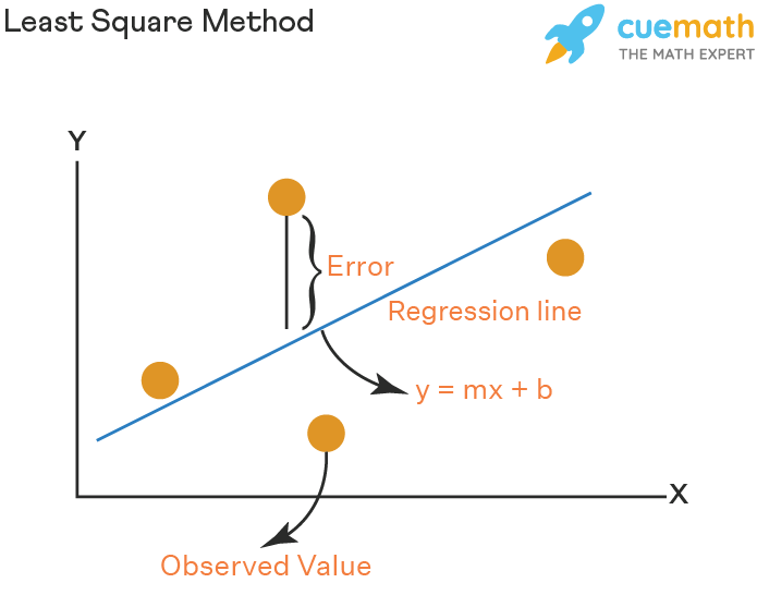
Method: least square. Find the best line by minimizing the the sum of the squared errors.
-
Degree of freedom: number of independent variables
-
Covariance Type: typically nonrobust, which means there is no elimination of data to calculate the covariance between features
-
R-squared: One of the most important number in the table, also known as the coefficient of determination. R-squared represents the proportion of variance in the dependent variable that is explained by the independent variables. It ranges from 0 to 1, with higher values indicating a better fit. For example, 0.793 means the model explains 79.3% of the change in y variable
\[\begin{equation} R^2 = 1-\dfrac{ \sum(y_i - \hat{y}_i)^2}{\sum(y_i - \bar{y})^2} \end{equation}\]y~i~ = observed values, ŷ= predicted values, ȳ = mean of the observed values
-
Adj. R-squared: Similar to R-squared but it penalizes the addition of unnecessary predictors. Consequently, a diminished adjusted score may indicate that some variables are not contributing to your model’s R-squared.
-
F-statistic and Prob (F-statistic): The F-test indicates whether your linear regression model provides a better fit than a model with all parameters equal to zero. $H_0:\beta_1=\beta_2=⋯=\beta_i=0$ A small p-value (typically less than 0.05) indicates that the model as a whole is significant.
-
Log-Likelihood 1: The natural logarithm of the likelihood. The likelihood is a function that tells the probability of observing the data given the model parameters, it is a product of probability density functions 𝑓~𝜃~. $L(𝜃 𝑋)=∏_{𝑖=1}^𝑛𝑓_𝜃(𝑋_𝑖)$. Log-likelihood values cannot be used alone as an index of fit because they are a function of sample size but can be used to compare the fit of different coefficients. - AIC and BIC: Akaike Information Criterion (AIC) and Bayesian Information Criterion (BIC) are both related to log-likelihood functions. They balance model complexity with goodness of fit, helping to prevent overfitting. Lower AIC or BIC values indicate better model fit, while taking into account the number of parameters in the model.
Section II - Coefficients
-
Coefficients : In a classic linear formula $y = mx+\beta$ , coefficients is our β
-
Std err: The standard error is the (estimated) standard deviation of the sampling distribution of 𝛽̂ $SE = \frac{\sigma}{\sqrt{n}}$ . The standard error quantifies the uncertainty or variability in this estimated coefficient. A smaller standard error indicates higher precision, meaning that the estimated coefficient is likely closer to the true population value.
-
t: The t-statistic, which tests the null hypothesis that the coefficient is equal to zero. Based on that test we may decide whether x is a useful (linear) predictor of y.
-
**P> t :** Another important feature in the summary table. The p-value is associated with the t-statistic. A small p-value indicates that the coefficient is statistically significant. A p-value of 0.05 or lower is generally considered statistically significant. 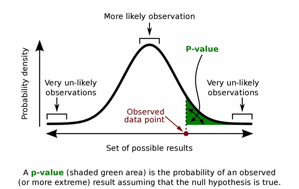
- [0.025 0.975]: The 95% confidence interval for the coefficient. It provides a range of plausible values for the true coefficient.
Section III - Shape of distribution
-
Omnibus, Prob(Omnibus): The Omnibus test measures the normality of the residuals with 0 meaning perfect, and the associated p-value (Prob(Omnibus)) indicates whether the test is statistically significant.
-
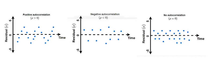
Durbin-Watson: It is a test to detect autocorrelations in the residuals. Its scale spans from 0 to 4, where values proximate to 2 signify an absence of autocorrelation, 0 indicates positive autocorrelation, and 4 implies negative autocorrelation. Autocorrelation occurs when the errors (residuals) of a regression model exhibit patterns with themselves at different lags, and the residuals are not independent of each other. One common approach to visually assess autocorrelation is by plotting residual plots, as depicted in the accompanying images below.
-
Jarque-Bera (JB) and Prob(JB): Similar to the Omnibus test, the Jarque-Bera test evaluates the normality of the residuals. The p-value (Prob(JB)) indicates whether the test is statistically significant.
-
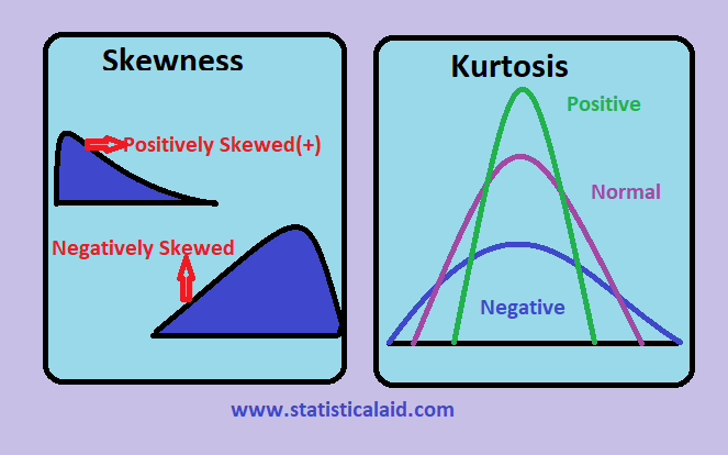
Skewness and Kurtosis: Skewness measures the asymmetry of the distribution and Kurtosis is a measure of whether the data are heavy-tailed or light-tailed relative to a normal distribution.
Conclusion
Interpreting a Statsmodels summary table requires a solid understanding of statistical concepts and an appreciation for the nuances of the model being analyzed. By carefully examining the coefficients, p-values, confidence intervals, and diagnostic statistics provided in the summary table, you can gain valuable insights into the relationships between variables and the overall performance of the model. However, it’s essential to remember that statistical analysis is not an exact science, and interpretation should always be accompanied by critical thinking and consideration of the context in which the analysis was conducted. With practice and experience, you can become proficient in interpreting Statsmodels summary tables and using them to inform data-driven decisions.
Happy modeling!
Reference
-
https://www.statlect.com/glossary/log-likelihood by Log-likelihoodby Marco Taboga PhD. ↩